X-ray Attenuation
The probability of survival (\( s \)) of an X-ray photon which penetrates an object is given by an exponential function of the objects "mass thickness" (\(x=\rho t\)). An object of either double thickness or double density will have a double mass thickness \( 2x = \rho (2 t) = (2\rho) t \). So what happens to a beam of X-rays shining through the object? If the initial X-ray intensity (total photon count) is given by \(I_0\) and the final intensity is given by \(I\), then the change in intensity of the X-ray beam is described by Eq (1). Multiply the initial photon count by the probability of survival to find the final photon count. The rate of exponential attenuation for different materials at different X-ray energy levels is measured by the National Institute of Standards and Technology (
NIST).
$$
\begin{align*}
I = I_0 s = I_0 e^{-(\mu / \rho) x}\tag{Eq 1}
\end{align*}
$$
\(\mu\) \([\text{cm}^{-1}]\) = attenuation rate
\(\rho\) \([g/\text{cm}^3]\) = density
\(x\) \([g/\text{cm}^2]\) = mass thickness
(\( 0 < s < 1 \)). For example if \( \mu = \rho = x = 1 \), Eq (1) simplifies to \(I = I_0 e^{-1} = I_0 \cdot 0.3679\). So if 100 photons enter the object 36.79 of them will survive.
Eulers Number
If you create a \(10 \times 10 \) matrix of cells and make a part of each cell opaque so that it scatters \(1/10\)th of the penetrating photons, then a beam of photons penetrating 10 cells in a row will have a survival probability of \((1-1/10)^{10} = 0.3487\). If you make an \(n \times n \) matrix (and if n is large), then \(1/e\) photons will survive.
$$
\begin{align*}
\left(1-\frac{1}{n}\right)^n = \frac{1}{e} = 0.3679
\end{align*}
$$
By definition the exponential function \( e^x = \left ( 1 + \frac{x}{n} \right )^n \) for large n.
Basis Approximation
Selecting 15 rows on the NIST tables from 3 [keV] to 150 [keV] a vector may be created which contains the attenuation rates for a particular element on the periodic table. Let \( M_i \) represent this column vector for the \(i^\text{th}\) element (\(i = Z\), Atomic Number). The matrix \(A\) may be formed from the first 10 elements as shown below.
$$
\begin{align*}
A &=
\begin{bmatrix}
M_1^\text{T} \\
\vdots\\
M_{10}^\text{T} \\
\end{bmatrix} \\
\end{align*}
$$
If \(\mathcal{E}\) represents the mean point of the \(M_i\)'s, then for normalization \(\bar{A} = A - \mathcal{E} \). Now let the unit vector \( v_i \) represent the \(i^{th}\) singular vector of \(\bar{A}\), and \(\sigma_i\) represent the \(i^{th}\) singular value. Eq (2) provides a basis \( \underset{(15 \times 3)}{\Lambda} \) of orthogonal singular vectors which approximates \((\mu / \rho ) x \) within the span of the first 10 elements.
$$
\begin{align*}
\text{std}(A v_i) &= \sqrt{\frac{\left\|\bar{A} v_i \right\|^2}{n-1}} = \sqrt{\frac{\sigma_i^2}{n-1}}\\
\bar{A} v_i &= \sigma_i u_i
\end{align*}
$$
$$
\begin{align*}
(\mu / \rho ) x = \begin{bmatrix} v_1 , v_2 , v_3 \end{bmatrix} y + \mathcal{E}&= \Lambda y + \mathcal{E}\tag{Eq 2}
\end{align*}
$$
The first three singular vectors have standard deviations of 157.66, 1.45 and 0.15 respectively (higher values are near zero). The Matlab code and plot for Figure 1 is given in Appendix A.
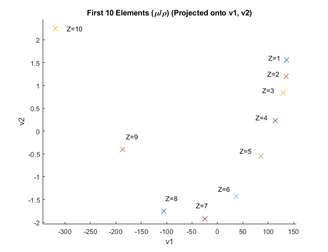
Figure 1
Eigenvalue/Singular Value Relationship
Define \(\lambda_i\) to be the standard deviation of \(A v_i\), for \(v_i\) of unit length.
$$
\begin{align*}
\text{std}(A v_i ) &= \sqrt{\frac{\|\bar{A} v_i \|^2}{n-1}} = \lambda_i\\
\lambda_i^2 &= \frac{\sigma_i^2}{n-1}\\
\\
\lambda_i^2 &= \frac{(\bar{A} v_i)^\text{T} (\bar{A} v_i)}{n-1} = \frac{v_i^\text{T}\bar{A}^\text{T} \bar{A} v_i}{n-1} = v_i^\text{T} C v_i\\
\end{align*}
$$
$$
\begin{align*}
C v_i &= \lambda_i^2 v_i
\end{align*}
$$
or you could say:
$$
\begin{align*}
(\bar{A}^\text{T} \bar{A}) v_i = \sigma_i^2 v_i
\end{align*}
$$
They both describe the same eigenvectors \(v_i\).
Composite Materials
The Z fractions by weight are given by the
NIST (mixtures) tables. \( W_i \) is the scalar mass fraction of the \(i^{th}\) Atomic Number in a mixture of different elements. Examples from the NIST tables and the Basis coordinates \(y\) from Eq (2) are given for Water and Teflon below. Plots are given in Figures 2 and 3. (See Appendix A for the Matlab code)
$$
\begin{align*}
\left(\mu / \rho \right) = A^{\text{T}} \begin{bmatrix} W_1 \\ W_2 \\ \vdots \\ W_n \end{bmatrix} = A^{T} W
\end{align*}
$$
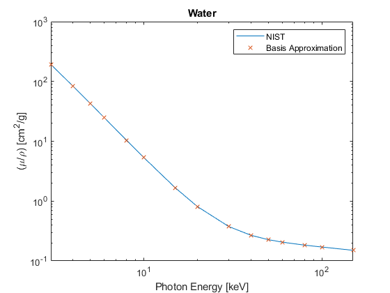
Figure 2
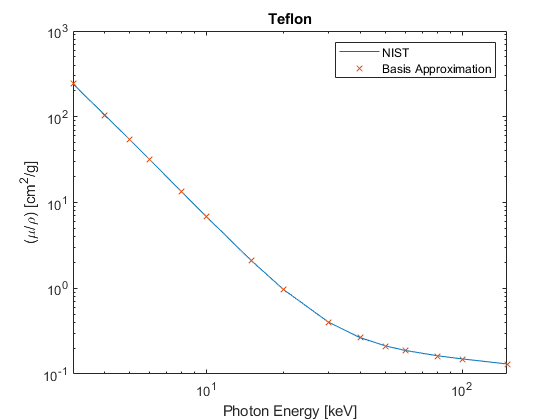
Figure 3
Water, Liquid
Z:(mass fraction)
1: 0.111898
8: 0.888102
y =
-78.5260
-1.3866
-0.0973
Teflon
6: 0.240183
9: 0.759818
y =
-133.2042
-0.6488
-0.0016
Mass Fractions
Mass fractions are calculated by summing the Atomic Mass Units [amu] from the
Periodic Table.
Z:(AMU)
1: 1.0080 (H)
6: 12.011 (C)
8: 15.999 (O)
9: 18.998 (F)
$$
\begin{align*}
\text{mass}(H_2 O)&= 2(1.0080) + (15.999) = 18.0150 [\text{amu}]\\
\text{mass}(C_2 F_4) &=2(12.011) + 4(18.998) = 100.0140 [\text{amu}]
\end{align*}
$$
$$
\begin{align*}
\frac{2(1.0080) + (15.999)}{18.0150} = 0.1119 + 0.8881\\
\frac{2(12.011) + 4(18.998)}{100.0140} = 0.2402 + 0.7598
\end{align*}
$$
$$
\begin{align*}
1 [\text{amu}] = 1 \left [ \frac{g}{\mathcal{N}} \right ]\\
\mathcal{N} = 6.022e23 (\text{atoms})
\end{align*}
$$
If you have \(\mathcal{N}\) atoms of Carbon-12:
$$
\begin{align*}
\mathcal{N} \cdot 12 [\text{amu}] = \mathcal{N} \cdot 12 \left[ \frac{g}{\mathcal{N}} \right] = 12g
\end{align*}
$$
If you have \(\mathcal{N}\) atoms of Carbon-13:
$$
\begin{align*}
\mathcal{N} \cdot 13 [\text{amu}] =\mathcal{N} \cdot 13 \left[ \frac{g}{\mathcal{N}} \right] = 13g
\end{align*}
$$
Carbon in nature has mass fractions of \(.99 (12) + .01 (13) = 12.01\). (
Isotopes of carbon)
Cubic Polynomial Z
An elements distance from the mean along the \(v_1\) singular vector is proportional to \(Z^3\). Figure 4 shows the interpolation.
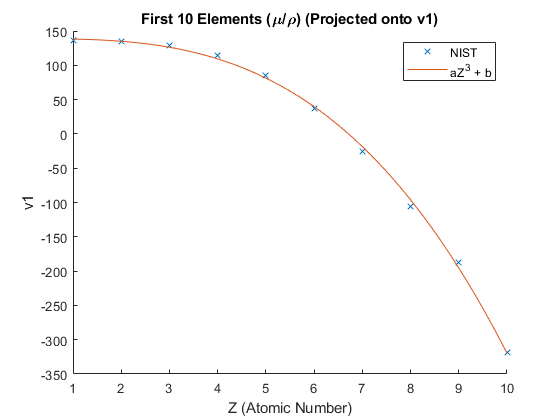
Figure 4
Let \(X=Z^3\) to simplify the plot. (Figure 5) \(H_2 O\) is located using the mass fractions given by NIST.
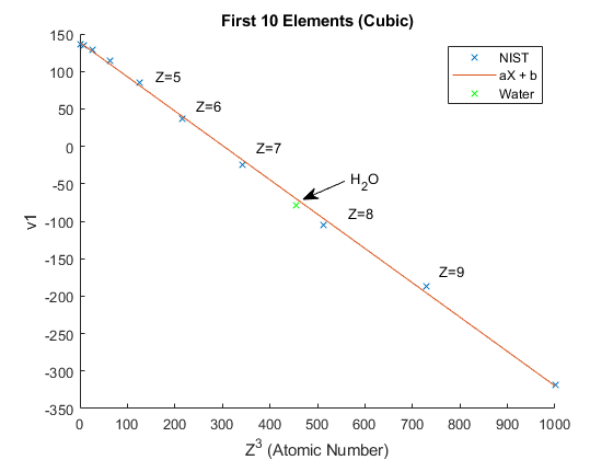
Figure 5
Weighted sums of the Atomic Number give the effective Z. For example water contains Z=1 and Z=8. Taking a weighted sum using the mass fractions gives an effective Z of 7.69
$$
\begin{align*}
Z_{\text{eff}}^3 &= 0.111898 (1)^3 + 0.888102 (8)^3 = 454.82 \\
Z_{\text{eff}} &= \sqrt[3]{454.82} = 7.69
\end{align*}
$$
This article:
(Zeff) weights mixtures using the electron fraction instead of the mass fraction. So for example Hydrogen has a weight of 2 electrons and Oxygen just 8. This is a different method than the one used by NIST to produce the attenuation spectra of mixtures.
$$
\begin{align*}
Z_{\text{eff}}^3 &= 0.2 (1)^3 + 0.8 (8)^3 = 409.8 \\
Z_{\text{eff}} &= \sqrt[3]{409.8} = 7.43
\end{align*}
$$
Regardless of how the mass or electron fractions are calculated, the end result is some linear combination of basis materials. The \(\Lambda\) Basis includes all possible materials under consideration and contains a minimal set of linearly independent basis vectors as its columns.
Attenuation Units
The attenuation units (AU) can be expressed in \(\Lambda\) Basis coordinates. The dimension could be increased if higher Z materials are needed. Metals require higher dimensional representations (More than 3) but only the first 10 elements were used in this post.
$$
\begin{align*}
I &= I_0 e^{-( \Lambda y + \mathcal{E} )}\\
\text{AU} = -\text{ln} \left( I / I_0 \right) &= (\mu / \rho) x = \Lambda y + \mathcal{E}
\end{align*}
$$
Appendix A
Matlab Code - Singular Values (Figure 1)
%tabulate NIST attenuation rates [cm^2/g]
A = zeros(10,15);
for i = 1:10 %Z=1 through 10
A(i,:) = MU(i)'; %Load i'th element from NIST tables
end
%normalize by mean values
Ec = mean(A,1);
A = A-Ec;
%find first 3 singular vectors
[U,S,V] = svd(A);
v1 = V(:,1);
v2 = V(:,2);
v3 = V(:,3);
a1 = A*v1;
a2 = A*v2;
a3 = A*v3;
%standard deviations
s1 = std(a1)
s2 = std(a2)
s3 = std(a3)
figure
axes
hold on
for i = 1:10
plot(a1(i),a2(i),'x')
end
Results:
s1 = 157.6640
s2 = 1.4525
s3 = 0.1534
Matlab Code - Composite Materials (Figures 2,3)
%NIST X-ray beam energy levels [keV]
E = [3 4 5 6 8 10 15 20 30 40 50 60 80 100 150]'; %15 energy levels
%tabulate NIST attenuation rates [cm^2/g]
A = zeros(10,15);
for i = 1:10 %Z=1 through 10
A(i,:) = MU(i)'; %Load i'th element from NIST tables
end
Ec = mean(A,1);
Abar = A-Ec;
[U,S,V] = svd(Abar);
L = V(:,1:3);
M_water = 0.111898*MU(1) + 0.888102*MU(8); %NIST
y = L \ (M_water - Ec') %best coordinates
M_approx = L*y + Ec'; %Basis Approximation
Results:
y =
-78.5260
-1.3866
-0.0973
Matlab Code - Cubic Polynomial (figure 4)
%tabulate NIST attenuation rates [cm^2/g]
A = zeros(10,15);
for i = 1:10 %Z=1 through 10
A(i,:) = MU(i)'; %Load i'th element from NIST tables
end
Ec = mean(A,1);
Abar = A-Ec; %mean normalize
[U,S,V] = svd(Abar);
v1 = V(:,1);
x = (1:10)';
y = Abar*v1; %project onto first singular vector
x3 = x.^3;
B = [x3 ones(10,1)];
c = B\y %polynomial interpolation
X = linspace(1,10,100);
Y = c(1)*X.^3 + c(2);
figure
axes
hold on
plot(x,y,'x'); %along first singular vector
plot(X,Y); %Z cubed interpolation
Results:
c =
-0.4584
138.6715
Matlab Code - Zeff (figure 5)
%tabulate NIST attenuation rates [cm^2/g]
A = zeros(10,15);
for i = 1:10 %Z=1 through 10
A(i,:) = MU(i)'; %Load i'th element from NIST tables
end
Ec = mean(A,1);
Abar = A-Ec; %mean normalize
[U,S,V] = svd(Abar);
v1 = V(:,1);
x = (1:10)';
y = Abar*v1; %project onto first singular vector
Z3 = x.^3;
B = [Z3 ones(10,1)];
c = B\y; %polynomial interpolation
a = c(1);
b = c(2);
X = linspace(1,10^3,100);
Y = a*X+b;
figure
axes
hold on
plot(Z3,y,'x')
plot(X,Y)
%Water test
M_water = 0.111898*MU(1) + 0.888102*MU(8); %NIST
u_water = (M_water-Ec')'*v1 %project onto v1
%chemistry estimate
Zeff_3 = 0.111898*(1)^3 + 0.888102*(8)^3
Zeff = Zeff_3^(1/3)
plot(Zeff_3,u_water,'gx')
References
Seltzer, S.M., Hubbel, J.H. (1996)
NIST Standard Reference Database 126, Radiation Physics Division, PML, NIST (Last update: 2004)