Density Images
(Material)[g/cm^3]
1) Teflon 2.20 PTFE
2) Al 2.70 Aluminum 6061
3) Steel 7.87 AISI 1018
4) Ti 4.43 Titanium 5
Mass Attenuation Coefficients

Figure 1
1) Teflon
6: 0.240183
9: 0.759818
2) Aluminium 6061
12: 0.012
13: 0.969
14: 0.008
26: 0.007
29: 0.004
3) Steel (AISI 1018)
6: 0.0017
25: 0.0075
26: 0.9908
4) Titanium (5)
13: 0.06
22: 0.90
23: 0.04
Matlab Code - Mass Attenuation Coefficients (Figure 1)
E = [3 4 5 6 8 10 15 20 30 40 50 60 80 100 150]'; %15 energy levels
%Density [g/cm^3]
R_tf = 2.20;
R_al = 2.70;
R_st = 7.87;
R_ti = 4.43;
%MU
M_tf = 0.240183*MU(6) + 0.759818*MU(9);
M_al = .969*MU(13)+.012*MU(12)+.008*MU(14)+.007*MU(26)+.004*MU(29);
M_st = .9908*MU(26) + .0075*MU(25) + .0017*MU(6);
M_ti = .90*MU(22) + .06*MU(13) + .04*MU(23);
figure
loglog(E,M_tf);
hold on
loglog(E,M_al);
loglog(E,M_st);
loglog(E,M_ti);
Effective \(\mu\)
For two objects of length \(t\).
$$
\begin{align*}
\text{AU} = \left ( M_1 \rho_1 + M_2 \rho_2 \right ) t = \mu_\text{eff} t
\end{align*}
$$
Energy-Fluence
The Energy-Fluence vector (\(\Psi\)) gives the source and detector response for an energy integrating detector. \(\sum_i \Psi_i = 1\) This is a vector form of the notation used by
Lu 2019. Eq (1) gives the measured data \(d\) as a function of length \(t\).
$$
\begin{align*}
d = \frac{I}{I_0} = \Psi^T e^{- \mu_\text{eff} t} \tag{Eq 1}
\end{align*}
$$
Energy-Fluence weights are selected proportional to bin width for a flat energy integrating detector.
Energy-Fluence
[keV] [bin width]
3 1
4 1
5 1
6 1.5
8 2
10 3.5
15 5
20 7.5
30 10
40 10
50 10
60 15
80 20
100 35
150 50
Loss of Dimensionality
Let \(\text{AU} = -\text{ln}(d)\). The plot in Figure (2) shows the relationship to \(x\).
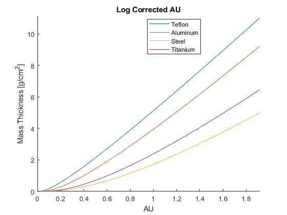
Figure 2
Matlab Code - Loss of Dimensionality (Figure 2)
E = [3 4 5 6 8 10 15 20 30 40 50 60 80 100 150]'; %15 energy levels
Psi = [1 1 1 1.5 2 3.5 5 7.5 10 10 10 15 20 35 50]'; %bin width
Psi = Psi/sum(Psi); %normalize to 1
%Density [g/cm^3]
R_tf = 2.20;
R_al = 2.70;
R_st = 7.87;
R_ti = 4.43;
%Mass Attenuation Coefficients
M_tf = 0.240183*MU(6) + 0.759818*MU(9);
M_al = .969*MU(13)+.012*MU(12)+.008*MU(14)+.007*MU(26)+.004*MU(29);
M_st = .9908*MU(26) + .0075*MU(25) + .0017*MU(6);
M_ti = .90*MU(22) + .06*MU(13) + .04*MU(23);
%Energy-Fluence
t = linspace(0,5,1000);%lengths [cm]
d_tf = sum(Psi.*exp(-M_tf*R_tf.*t));
d_al = sum(Psi.*exp(-M_al*R_al.*t));
d_st = sum(Psi.*exp(-M_st*R_st.*t));
d_ti = sum(Psi.*exp(-M_ti*R_ti.*t));
%Wishful Thinking
AU_tf = -log(d_tf);
AU_al = -log(d_al);
AU_st = -log(d_st);
AU_ti = -log(d_ti);
X_tf = R_tf*t;
X_al = R_al*t;
X_st = R_st*t;
X_ti = R_ti*t;
figure
axes
hold on
plot(AU_tf, X_tf)
plot(AU_al, X_al)
plot(AU_st, X_st)
plot(AU_ti, X_ti)
For a monoenergetic 80 keV source the Energy-Fluence spectrum becomes:
Energy-Fluence
[keV] [weight]
3 0
4 0
5 0
6 0
8 0
10 0
15 0
20 0
30 0
40 0
50 0
60 0
80 1
100 0
150 0
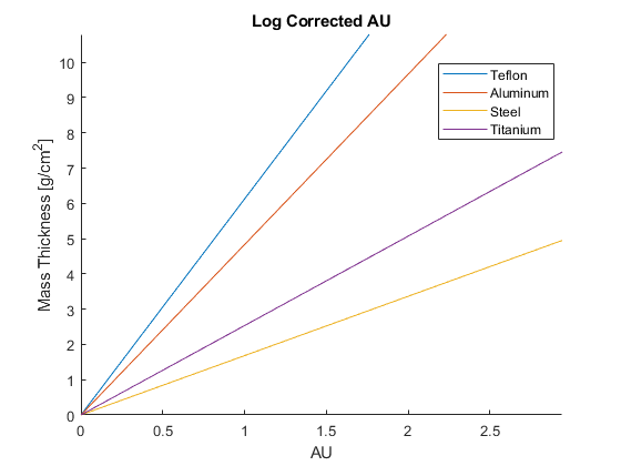
Figure 3