Fundamental Frequency

The fundamental frequency of a note bowed on a stringed instrument (the Viola) may be extracted by selecting the lowest frequency peak from a series of overtones. An alternate way of extracting the fundamental frequency is also discussed for cases where the lowest frequency peak can not be read directly. The terms overtones and harmonics are used interchangeably in this post.

Algorithm Summary

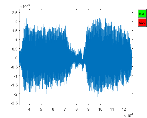
1.) Crop the raw time domain audio data to the region of interest. In this case the section where the note is being played.
2.) Take the FFT. Use fftshift in Matlab so the middle frequency is 0.
3.) Generate the frequency axis from the negative half max frequency to the positive half max frequency. (-fs/2 to fs/2). (fs is the sample frequency of the audio recorder)
4.) Window the frequency axis between 100 and 2000 Hz. This can be done with a mask in matlab.
5.) Find local maxima of the frequency domain signal (above a cutoff height, "MinProminence" using the islocalmax function).
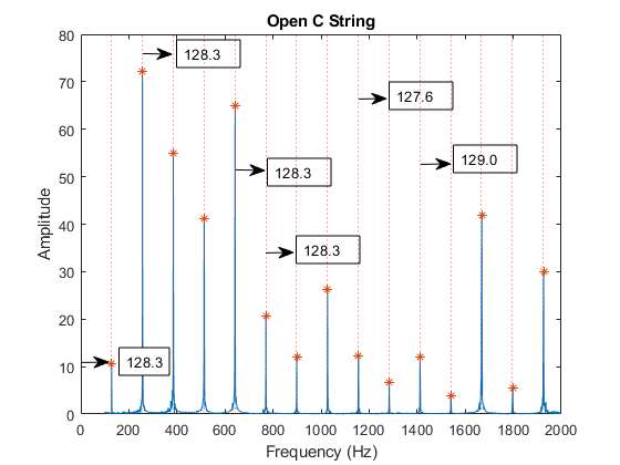
6.) Select the lowest peak with respect to frequency. This is the Fundamental Frequency.

Matlab code is included in Appendices 1 and 2. In Appendix 1 the code for recording a segment of audio data in matlab is given. In Appendix 2 the code for extracting the fundamental frequency is given.

Overtones

If the fundamental frequency is F, overtones will be located at frequencies 2F, 3F, 4F,etc... This is verified by selecting the lowest fundamental and multiplying by i = 1:length(xp) (where xp is the vector containing the frequency of the peaks.) The dotted red lines on the plots below show the expected location of the overtones. The fft plot also shows peaks at those locations.

$$ \begin{align*} F_3-F_2 &= 3F-2F\\ 3F-2F &= (3-2) F = F \end{align*} $$ The equation above shows that if the 2nd and 3rd harmonics are measured the fundamental frequency F may be extracted by taking the difference between them. This method is described in the discussion section below.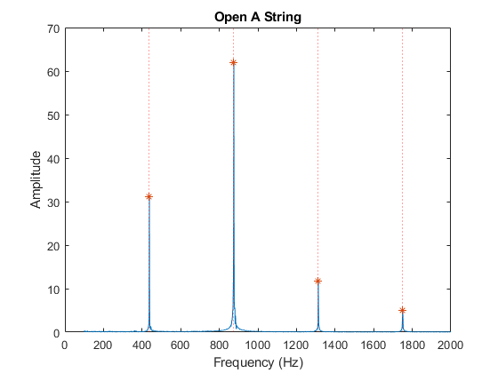

Note on Pitch Class

When converting to the Pitch Class (see 3_29_23) using a modulo 12 representation the first harmonic is equivalent to the fundamental frequency.(So would the 4th,8th,\(2^n\) etc...) Meaning Open C is equivalent to middle C with respect to the pitch class.
$$ \begin{align*} P(261.6) &= 12\cdot\log_2\left(\frac{261.6}{440}\right) +9 \quad (\text{mod 12}) \approx 0.0\\ P(130.8) &= 12\cdot\log_2\left(\frac{130.8}{440}\right) +9 \quad (\text{mod 12}) \approx 0.0 \end{align*} $$

Plots

Discussion

The overtones of the fundamental frequency can be read off like a ruler. The distance between them in frequency space is (approximately) the fundamental frequency. In Figure 1 below some of the distances are calculated by subtracting adjacent peaks.

If it is desired to read off the fundamental frequency of a recording of a bowed note that is obscured by noise in the lower part of the frequency domain or for whatever reason the fundamental can not be read by selecting the minimum peak, its value can be determined by averaging together the difference between several of the adjacent overtones. It would make the most sense when a set of measurements are taken to use the median of the distance between overtones to remove extraneous peaks such as the one in 5th harmonic of the open d string data plotted above.

In a quick test the 5th through 8th peaks (from the open C data) are used in this way to calculate the fundamental rather than reading the min(xp). This returns 128.291 which is identical with the fundamental which in this case is 128.291 as well. The matlab code to do this is given below.

b = xp(5:8);
median(diff(b))

Figure 1

Appendix 1

The following matlab code creates a simple audio recorder with a start and a stop button as shown in the image below.

%%%%%%%%%%%%%%%%%%%%%%%%%%%%%%%%%%
%Set up figure
%%%%%%%%%%%%%%%%%%%%%%%%%%%%%%%%%%
f1 = figure;
f1.Position = [0 0 500 400]; %set window position
a1  = axes(f1); %axes for plotting

%%%%%%%%%%%%%%%%%%%%%%%%%%%%%%%%%%
%Set up audiorecorder
%%%%%%%%%%%%%%%%%%%%%%%%%%%%%%%%%%
fs = 44100; %sample frequency
nBits = 16;
nChannels = 1; 
ID = -1; %default audio input device

recObj = audiorecorder(fs,nBits,nChannels,ID);
recObj.TimerPeriod = .1;
recObj.TimerFcn = @(s,e) update_plot(a1, recObj);

%%%%%%%%%%%%%%%%%%%%%%%%%%%%%%%%%%
%start/stop buttons
%%%%%%%%%%%%%%%%%%%%%%%%%%%%%%%%%%
b1 = uicontrol(f1);
b1.Style = 'pushbutton';
b1.String = 'start';
b1.BackgroundColor = 'green';
b1.Position = [500-30 400-60 30 30];
b1.Callback = @(s,e) record(recObj); %start recording

b2 = uicontrol(f1);
b2.Style = 'pushbutton';
b2.String = 'stop';
b2.BackgroundColor = 'red';
b2.Position = [500-30 400-90 30 30];
b2.Callback = @(s,e) stop(recObj); %stop recording

%%%%%%%%%%%%%%%%%%%%%%%%%%%%%%%%%%
%recObj Callback function
%%%%%%%%%%%%%%%%%%%%%%%%%%%%%%%%%%
function update_plot(a1, recObj)
    y = getaudiodata(recObj); %get the audio data
    plot(a1,y); %plotaudio data
end

Appendix 2

The following matlab code loads the audio data previously saved from the output of (A = getaudiodata(recObj)). The fundamental frequency is given by min(xp).

load("OpenStrings.mat");

fs = 44100; %sample frequency (Hz)

%crop
A = A(160000:200000);
D = D(138000:200000);
G = G(124000:185000);
C = C(145000:211000);

%extract fundamental frequency  
Signal = A; %start with open string A
sound( Signal, fs, 16 ); %play the sound

F = abs(fftshift(fft(Signal)));
x = linspace(-fs/2,fs/2, length(Signal)); %frequency domain x-labels

mask = (x>100) & (x<2000); %min and max frequency (Hz)
F = F(mask);
x = x(mask)';

p = islocalmax(F,"MinProminence",3.5); %get peaks
Fp = F(p); %amplitude
xp = x(p); %frequency

min(xp)

cla
plot(x,F);
hold on;
plot(xp,Fp,'*');
xlim([0 2000]);

for i=1:length(xp)%plot overtones as a dotted line
    h = xp(1)*i;
    xline(h,'r:');
end