Understanding the FFT
The following examples are based on the book by Anders E. Zonst. "Understanding the FFT, Second Edition, Revised" (1995, 2000) The code in this book is written in BASIC. For the FFT section I use the algorithm described in "Linear Algebra with Applications, Ninth Edition" (2015, 2006) by Steven J. Leon. The examples below are implemented in the Matlab programming language.
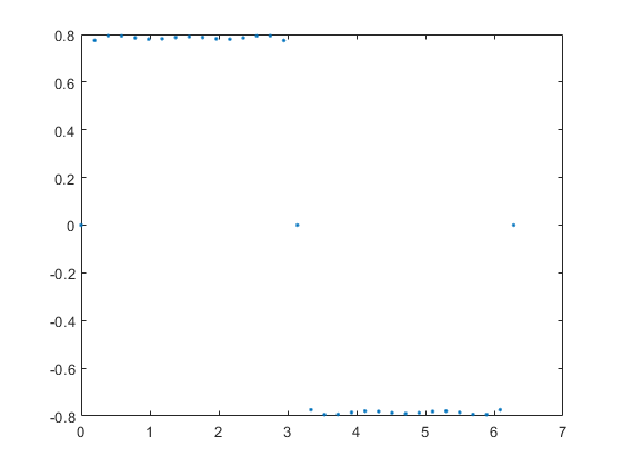
Square Wave
Let \(x \in \left( 0:\frac{\pi}{16}:2 \pi \right) \) radians. In this example i represents the harmonic number. So the sum of all odd harmonics produces a square wave, all harmonics produce a sawtooth and there are many other waveforms that can be produced like this.
$$
\begin{equation}
f(x) = \sum_{i \in (1, 3, 5 \cdots)} \frac{\sin(ix)}{i}
\end{equation}
$$
Matlab Code
n = 101;
x = 0:pi/16:2*pi;
y = zeros(size(x));

for i=1:2:n
    y = y + sin(i*x)/i;
end

plot(x, y, '.')
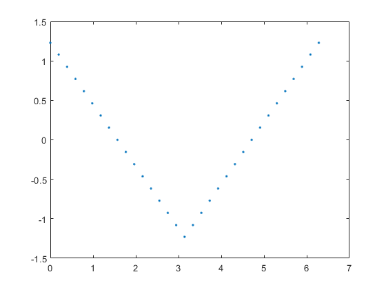
Triangle Wave
Modify the square wave by changing sine to cosine and dividing instead by \(i^2\).
Let \(x \in \left( 0:\frac{\pi}{16}:2 \pi \right) \) radians.
$$
\begin{equation}
f(x) = \sum_{i \in (1, 3, 5 \cdots)} \frac{\cos(ix)}{i^2}
\end{equation}
$$
Matlab Code
n = 101;
x = 0:pi/16:2*pi;
y = zeros(size(x));

for i=1:2:n
    y = y + cos(i*x)/(i^2);
end

plot(x, y, '.')
DFT
For an example of the DFT generate a triangle wave for a test function by summing cosine functions up to the 7th harmonic.
Let \(x \in (0:15)\frac{2 \pi}{16} \) radians.
$$
\begin{equation}
\underset{(1 \times 16)}{y} = \sum_{i \in (1, 3, 5, 7)} \frac{\cos(ix)}{i^2}
\end{equation}
$$
Recover the amplitude of the \(i^\text{th}\) harmonic number \(\frac{1}{i^2}\) by multiplying the test frequency vector by \(y^{\text{T}}\) and dividing by the total number of points.
$$
\begin{align*}
\text{fc}(i) &= \cos(ix) \cdot y^{\text{T}}\cdot \frac{1}{16}\\
\text{fs}(i) &= \sin(ix) \cdot y^{\text{T}}\cdot \frac{1}{16}
\end{align*}
$$
You can verify that the amplitude of the 7th harmonic of the cosine function, fc(7) is equal to exactly half \(\frac{1}{7^2}=0.0204\). The recovered amplitudes appear twice. First at fc(7) = 0.0102 and again at fc(9) = 0.0102 which gives both halves of 0.0204. Components 9 through 15 are mirror images of components 1 through 7. ("The two halves of the spectrum are symetrical about the Nyquist frequency except that the sine components are the negatives of each other", Page 43 Zonst)
Matlab Code
%%%%%%%%%%%%%%%%%%%%%%%%%%%%%%%%%%
%generate function y(x)
%%%%%%%%%%%%%%%%%%%%%%%%%%%%%%%%%%
x = (0:15)*2*pi/16; %radians
y = zeros(1,16);

for i=1:2:7
    y = y +cos(i*x)/(i^2); %triangle wave
end

%%%%%%%%%%%%%%%%%%%%%%%%%%%%%%%%%%
%DFT
%%%%%%%%%%%%%%%%%%%%%%%%%%%%%%%%%%
fc = @(i) cos(i*x) * y' /16; %recover cosine components
fs = @(i) sin(i*x) * y' /16; %recover sine components


%%%%%%%%%%%%%%%%%%%%%%%%%%%%%%%%%%
%Printing
%%%%%%%%%%%%%%%%%%%%%%%%%%%%%%%%%%
fprintf("i \t fc(i) \t\t fs(i) \n");
for i=0:15
    fprintf("%d \t % .4f \t % .4f \n", i, fc(i), fs(i));
end
Output
i 	  fc(i) 	  fs(i)
0 	 -0.0000 	  0.0000
1 	  0.5000 	  0.0000
2 	 -0.0000 	 -0.0000
3 	  0.0556 	 -0.0000
4 	 -0.0000 	  0.0000
5 	  0.0200 	  0.0000
6 	 -0.0000 	  0.0000
7 	  0.0102 	  0.0000
8 	  0.0000 	  0.0000
9 	  0.0102 	  0.0000
10 	  0.0000 	  0.0000
11 	  0.0200 	 -0.0000
12 	  0.0000 	 -0.0000
13 	  0.0556 	  0.0000
14 	  0.0000 	 -0.0000
15 	  0.5000 	 -0.0000
Inverse DFT
The Inverse DFT sums together all the harmonics of sine and cosine at the correct amplitudes to recover the original function.
In this example only cosine functions have nonzero amplitudes but in general both are used.
$$
\begin{equation}
\underset{(1 \times 16)}{z} = \sum_i \text{fc}(i) \cos(ix) + \text{fs}(i) \sin(ix)
\end{equation}
$$
Matlab Code
%%%%%%%%%%%%%%%%%%%%%%%%%%%%%%%%%%
%generate function y(x)
%%%%%%%%%%%%%%%%%%%%%%%%%%%%%%%%%%
x = (0:15)*2*pi/16; %radians
y = zeros(1,16);


for i=1:2:7
    y = y +cos(i*x)/(i^2); %triangle wave
end

%%%%%%%%%%%%%%%%%%%%%%%%%%%%%%%%%%
%DFT
%%%%%%%%%%%%%%%%%%%%%%%%%%%%%%%%%%
fc = @(i) cos(i*x) * y' /16; %recover cosine components
fs = @(i) sin(i*x) * y' /16; %recover sine components

%%%%%%%%%%%%%%%%%%%%%%%%%%%%%%%%%%
%Inverse DFT
%%%%%%%%%%%%%%%%%%%%%%%%%%%%%%%%%%
z = zeros(1,16);

for i=0:15
    z = z + fc(i)*cos(i*x) + fs(i)*sin(i*x);
end

%%%%%%%%%%%%%%%%%%%%%%%%%%%%%%%%%%
%Printing
%%%%%%%%%%%%%%%%%%%%%%%%%%%%%%%%%%
fprintf(" x \t\t\t  z(x) \t\t  y(x) \n");
for t=1:16
    fprintf("% .4f \t % .4f \t % .4f \n", x(t), z(t), y(t));
end
Vector z below recovers the test function y.
Output
 x 		  z(x) 		  y(x)
 0.0000 	  1.1715 	  1.1715
 0.3927 	  0.9322 	  0.9322
 0.7854 	  0.6147 	  0.6147
 1.1781 	  0.3092 	  0.3092
 1.5708 	  0.0000 	  0.0000
 1.9635 	 -0.3092 	 -0.3092
 2.3562 	 -0.6147 	 -0.6147
 2.7489 	 -0.9322 	 -0.9322
 3.1416 	 -1.1715 	 -1.1715
 3.5343 	 -0.9322 	 -0.9322
 3.9270 	 -0.6147 	 -0.6147
 4.3197 	 -0.3092 	 -0.3092
 4.7124 	 -0.0000 	 -0.0000
 5.1051 	  0.3092 	  0.3092
 5.4978 	  0.6147 	  0.6147
 5.8905 	  0.9322 	  0.9322
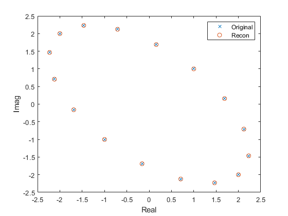
Switching to Complex Variables
Let j = \(\sqrt{-1}\). For testing complex valued functions an ellipse is generated in the complex plane.
Let \(x \in (0:15)\frac{2 \pi}{16} \) radians.
$$
\begin{equation}
\underset{(1 \times 16)}{y} = (\cos(x) + 2j\sin(x)) \cdot (1+1j)
\end{equation}
$$
The cosine and sine terms from the DFT can be represented by a single complex function using Eulers formula.
$$
\begin{align*}
\text{fc}(i) + j \text{fs}(i) &= \left(\cos(ix) + j \sin(ix) \right )\cdot y^{\text{T}} \frac{1}{16} = e^{jix}\cdot y^{\text{T}}\frac{1}{16}\\
f(i) &= e^{jix}\cdot y^{\text{T}}\frac{1}{16} \tag{Eq 1}
\end{align*}
$$
The same can be done for the inverse DFT.
$$
\begin{align*}
z &= \sum_i \left( \text{fc}(i) + j \text{fs}(i) \right) \left( \cos(ix) - j \sin(ix)\right) =\sum_i \left( \text{fc}(i) + j \text{fs}(i) \right) e^{-jix}\\
z &= \sum_i f(i) e^{-jix} \tag{Eq 2}
\end{align*}
$$
%%%%%%%%%%%%%%%%%%%%%%%%%%%%%%%%%%
%generate function y(x)
%%%%%%%%%%%%%%%%%%%%%%%%%%%%%%%%%%
x = (0:15)*2*pi/16; %radians
y = (cos(x)+2j*sin(x))*(1+1j); %ellipse

%%%%%%%%%%%%%%%%%%%%%%%%%%%%%%%%%%
%DFT
%%%%%%%%%%%%%%%%%%%%%%%%%%%%%%%%%%
F = @(i) exp(1j*i*x) * y.' /16;

%%%%%%%%%%%%%%%%%%%%%%%%%%%%%%%%%%
%Inverse DFT
%%%%%%%%%%%%%%%%%%%%%%%%%%%%%%%%%%
z = zeros(1,16);
for i=0:15
    z = z + F(i)*exp(- 1j*i*x);
end

cla
plot(y,'x')
hold on
plot(z,'o')
In the plot below the original complex valued function is compared with the inverse DFT of the DFT, the original function is recovered.
Cooley-Tukey FFT
The DFT described in Eq (1) can be represented by a single matrix multiplication where the test function \( y^{\text{T}} \) is of dimension \( (N\times 1) \) . Eq (3) gives the DFT. The matrix \(F_N\) is known as the Fourier matrix. If you are not comfortable with matrix multiplications I recommend reading the first few chapters of Leon.
$$
\begin{align*}
\omega_N &= e^{-\frac{2 \pi j}{N}}\\
F_N &=
\begin{bmatrix}
1 & 1 & 1 & 1 & \cdots & \omega_N^{0(N-1)} \\
1 & \omega_N & \omega_N^2 & \omega_N^3 & \cdots & \omega_N^{1(N-1)}\\
1 & \omega_N^2 & \omega_N^4 & \omega_N^6 & \cdots & \omega_N^{2(N-1)}\\
1 & \omega_N^3 & \omega_N^6 & \omega_N^9 & \cdots & \omega_N^{3(N-1)}\\
\vdots &\vdots & \vdots&\vdots & \ddots & \vdots \\
\omega_N^{(N-1)0} & \omega_N^{(N-1)1} & \omega_N^{(N-1)2} &
\omega_N^{(N-1)3}& \cdots & \omega_N^{(N-1)(N-1)}
\end{bmatrix}\\
d &= \begin{bmatrix}
f(0) \\
f(1) \\
f(2) \\
f(3) \\
\vdots \\
f(N-1)
\end{bmatrix} = F_N \cdot y^{\text{T}} \frac{1}{N} \tag{Eq 3}
\end{align*}
$$
The FFT (Fast Fourier Transform) is based on a refactorization of the Fourier Matrix of dimension \(N\times N\) into blocks of smaller Fourier Matrices of dimension \(N/2 \times N/2\). The factorization is given in eq (4) below.
\(\text{w}1 = \text{odd}(y^{\text{T}}) \)
\(\text{w}2 = \text{even}(y^{\text{T}}) \) gives the odd and even elements of \(y^{\text{T}}\)respectively.
\(D_N\) is a diagonal matrix whose \( n^{\text{th}}\) diagonal entry is \(\omega_{2N}^{n-1}\).
\begin{align*}
d &=
\begin{bmatrix}
F_{N/2} & D_{N/2} F_{N/2}\\
F_{N/2} & -D_{N/2} F_{N/2}
\end{bmatrix}
\begin{bmatrix}
\text{w}1 \\
\text{w}2
\end{bmatrix} \frac{1}{N} \tag{Eq 4}
\end{align*}
The code for the full FFT is given below.
%%%%%%%%%%%%%%%%%%%%%%%%%%%%%%%%%%
%generate function y(x)
%%%%%%%%%%%%%%%%%%%%%%%%%%%%%%%%%%
N = 16;
x = (0:N-1)*2*pi/N; %radians
y = zeros(1,N);

for i=1:2:16
    y = y +cos(i*x)/(i^2); %triangle wave
end

%%%%%%%%%%%%%%%%%%%%%%%%%%%%%%%%%%
%FFT
%%%%%%%%%%%%%%%%%%%%%%%%%%%%%%%%%%
y0 = y/N;
d = myfft(y0); %my fast recursive DFT
z = real(myfft(d));

%%%%%%%%%%%%%%%%%%%%%%%%%%%%%%%%%%
%Printing
%%%%%%%%%%%%%%%%%%%%%%%%%%%%%%%%%%
fprintf(" x \t\t\t  z(x) \t\t  y(x) \n");
for t=1:N
    fprintf("% .4f \t % .4f \t % .4f \n", x(t), z(t), y(t));
end

%%%%%%%%%%%%%%%%%%%%%%%%%%%%%%%%%%
%Full FFT
%%%%%%%%%%%%%%%%%%%%%%%%%%%%%%%%%%
function d = myfft(z)
	w = @(N) exp(-2*pi*1j/N); %Nth root of unity
	D = @(N) w(2*N).^(0:N-1)'; %offset

    N = length(z);

    if N == 1
        d = z; %base
    else
        w1 = z(1:2:end); %odd terms
        w2 = z(2:2:end); %even terms

        F1 = myfft(w1);
        F2 = myfft(w2);
        D1  = D(N/2);

        d = [F1+D1.*F2; F1-D1.*F2]; %apply rotation offset and sum
    end
end
The FFT applied twice gives the original function. This is a property of orthogonal matrices. The reconstruction of the function y(x) is plotted below. The results shown are identical.
Output
 x 		  z(x) 		  y(x)
 0.0000 	  1.2025 	  1.2025
 0.3927 	  0.9240 	  0.9240
 0.7854 	  0.6165 	  0.6165
 1.1781 	  0.3083 	  0.3083
 1.5708 	 -0.0000 	  0.0000
 1.9635 	 -0.3083 	 -0.3083
 2.3562 	 -0.6165 	 -0.6165
 2.7489 	 -0.9240 	 -0.9240
 3.1416 	 -1.2025 	 -1.2025
 3.5343 	 -0.9240 	 -0.9240
 3.9270 	 -0.6165 	 -0.6165
 4.3197 	 -0.3083 	 -0.3083
 4.7124 	  0.0000 	 -0.0000
 5.1051 	  0.3083 	  0.3083
 5.4978 	  0.6165 	  0.6165
 5.8905 	  0.9240 	  0.9240
The central mechanism of the FFT is the split into even and odd elements. In the following program a partial FFT is calculated by splitting the original DFT into even and odd elements. The plot below shows that the first even term is the first odd term rotated by the \( n^{\text{th}}\) root of unity raised to the \( i^{\text{th}}\)power (in this case 1). The rotation is accomplished by multiplication with the complex exponential.

The program below splits the test function into even and odd components and generates a partial FFT showing that the sum of the odd components with the same odd components multiplied by the \( n^{\text{th}}\) root of unity raised to the \( i^{\text{th}}\)power produces the same set of points as the original DFT.
%%%%%%%%%%%%%%%%%%%%%%%%%%%%%%%%%%
%generate function y(x)
%%%%%%%%%%%%%%%%%%%%%%%%%%%%%%%%%%
N = 16;
x = (0:N-1)*2*pi/N;
y = .5*sin(3*x);

%%%%%%%%%%%%%%%%%%%%%%%%%%%%%%%%%%
%DFT
%%%%%%%%%%%%%%%%%%%%%%%%%%%%%%%%%%
F = @(i) exp(1j*i*x) * y.' /N;

%%%%%%%%%%%%%%%%%%%%%%%%%%%%%%%%%%
%Partial FFT
%%%%%%%%%%%%%%%%%%%%%%%%%%%%%%%%%%
y0 = y/N;
w1 = y0(1:2:end)'; %odd elements
w2 = y0(2:2:end)'; %even elements

x1 = x(1:2:end); %odd elements
x2 = x(2:2:end); %even elements

F_odd = @(i) exp(1j*i*x1);

w = @(i) exp(1j*i*2*pi/N); %Nth root of unity
F2 = @(i) F_odd(i)*w1 + w(i)*F_odd(i)*w2;

%%%%%%%%%%%%%%%%%%%%%%%%%%%%%%%%%%
%Plots
%%%%%%%%%%%%%%%%%%%%%%%%%%%%%%%%%%
all_terms = @(i) exp(1j*i*x);
odd_terms = @(i) exp(1j*i*x1);
even_terms =@(i) exp(1j*i*x2);

cla
plot(odd_terms(1),'x')
hold on
plot(even_terms(1),'o')
plot(w(1),'^','MarkerSize',15)
axis equal